Author: Alan Murray / Source: How-To Geek

Pivot Tables are an amazing built-in reporting tool in Excel. While typically used to summarize data with totals, you can also use them to calculate the percentage of change between values. Even better: It is simple to do.
You could use this technique to do all kinds of things—pretty much anywhere you’d like to see how one value compares to another.
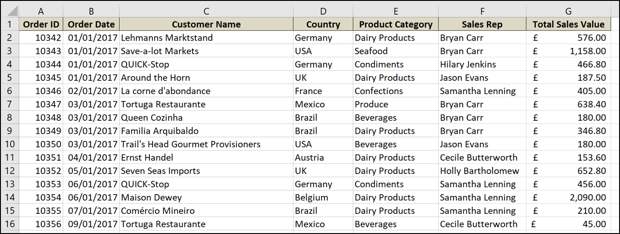
In this article, we’re going to use the straightforward example of calculating and displaying the percent by which the total sales value changes month by month.Here’s the sheet we’re going to use.

It’s a pretty typical example of a sales sheet that shows the order date, customer name, sales rep, total sales value, and a few other things.
To do all this, we’re first going to format our range of values as a table in Excel and we’re then going to create a Pivot Table to make and display our percentage change calculations.
Formatting the Range as a Table
If your data range is not already formatted as a table, we’d encourage you to do so. Data stored in tables have multiple benefits over data in cell ranges of a worksheet, especially when using PivotTables (read more about the benefits of using tables).
To format a range as a table, select the range of cells and click Insert > Table.

Check that the range is correct, that you do have headers in the first row of that range, and then click “OK.”
The range is now formatted as a table. Naming the table will make it easier to refer to in the future when creating PivotTables, charts, and formulas.
Click the “Design” tab under Table Tools, and enter a name in the box provided at the start of the Ribbon. This table has been named “Sales.”

You can also change the style of the table here if you want.
Create a PivotTable to Display Percentage Change
Now let’s get on with creating the PivotTable. From within the new table, click Insert > PivotTable.
The Create PivotTable window appears. It will have automatically detected your table. But you could select the table or range you want to use for the PivotTable at this point.

Group the Dates into…
The post How to Calculate Percentage Change with Pivot Tables in Excel appeared first on FeedBox.