Things have gotten freaky. A few years ago, Google showed us that neural networks’ dreams are the stuff of nightmares, but more recently we’ve seen them used for giving game character movements that are indistinguishable from that of humans, for creating photorealistic images given only textual descriptions, for providing vision for self-driving cars, and for much more.
Being able to do all this well, and in some cases better than humans, is a recent development.
Creating photorealistic images is only a few months old. So how did all this come about?Perceptrons: The 40s, 50s And 60s
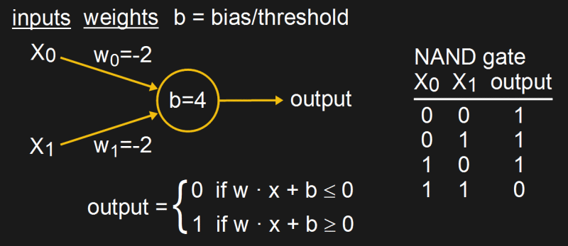
We begin in the middle of the 19th century. One popular type of early neural network at the time attempted to mimic the neurons in biological brains using an artificial neuron called a perceptron. We’ve already covered perceptrons here in detail in a series of articles by Al Williams, but briefly, a simple one looks as shown in the diagram.
Given input values, weights, and a bias, it produces an output that’s either 0 or 1. Suitable values can be found for the weights and bias that make a NAND gate work. But for reasons detailed in Al’s article, for an XOR gate you need more layers of perceptrons.
In a famous 1969 paper called “Perceptrons”, Minsky and Papert pointed out the various conditions under which perceptrons couldn’t provide the desired solutions for certain problems. However, the conditions they pointed out applied only to the use of a single layer of perceptrons. It was known at the time, and even mentioned in the paper, that by adding more layers of perceptrons between the inputs and the output, called hidden layers, many of those problems, including XOR, could be solved.
Despite this way around the problem, their paper discouraged many researchers, and neural network research faded into the background for a decade.
Backpropagation And Sigmoid Neurons: The 80s
In 1986 neural networks were brought back to popularity by another famous paper called “Learning internal representations by error propagation” by David Rummelhart, Geoffrey Hinton and R.J. Williams. In that paper they published the results of many experiments that addressed the problems Minsky talked about regarding single layer perceptron networks, spurring many researchers back into action.
Also, according to Hinton, still a key figure in the area of neural networks today, Rummelhart had reinvented an efficient algorithm for training neural networks. It involved propagating back from the outputs to the inputs, setting the values for all those weights using something called a delta rule.
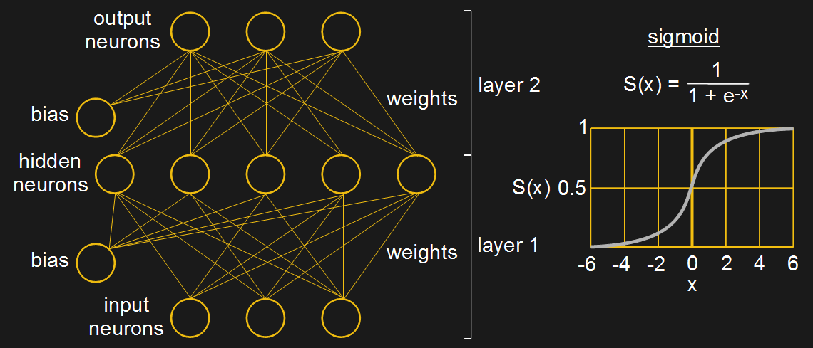
The set of calculations for setting the output to either 0 or 1 shown in the perceptron diagram above is called the neuron’s activation function. However, for Rummelhart’s algorithm, the activation function had to be one for which a derivative exists, and for that they chose to use the sigmoid function (see diagram).
And so, gone was the perceptron type of neuron whose output was linear, to be replaced by the non-linear sigmoid neuron, still used in many networks today. However, the term Multilayer Perceptron (MLP) is often used today to refer not to the network containing perceptrons discussed above but to the multilayer network which we’re talking about in this section with it’s non-linear neurons, like the sigmoid. Groan, we know.
Also, to make programming easier, the bias was made a neuron of its own, typically with a value of one, and with its own weights. That way its weights, and hence indirectly its value, could be trained along with all the other weights.
And so by the late 80s, neural networks had taken on their now familiar shape and an efficient algorithm existed for training them.
Convoluting And Pooling
In 1979 a neural network called Neocognitron introduced the concept of convolutional layers, and in 1989, the backpropagation algorithm was adapted to train those convolutional layers.
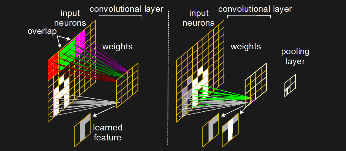
What does a convolutional layer look like? In the networks we talked about above, each input neuron has a connection to every hidden neuron. Layers like that are called fully connected layers. But with a convolutional layer, each neuron in the convolutional layer connects to only a subset of the input neurons. And those subsets usually overlap both horizontally and vertically. In the diagram, each neuron in the convolutional layer is connected to a 3×3 matrix of input neurons, color-coded for clarity, and those matrices overlap by one.
This 2D arrangement helps a lot when trying to learn features in images, though their use isn’t limited to images. Features in images occupy pixels in a 2D space, like the various parts of the letter ‘A’ in the diagram. You can see that one of the convolutional neurons is connected to a 3×3 subset of input neurons that contain a white vertical feature down the middle, one leg of the ‘A’, as well as a shorter horizontal feature across the top on the right. When training on numerous images, that neuron may become trained to fire strongest when shown features like that.
But that feature…
The post From 50s Perceptrons To The Freaky Stuff We’re Doing Today appeared first on FeedBox.